Documentation - NeuralLead Framework
The framework for 2nd and 3rd generation (Spike) neural networks.
Create, train and simulate neural networks quickly.
- Author: SimonJRiddix
- Last Update: 17 June, 2023
NeuralLead Maker
Installation
Follow these instructions to download NeuralLead Maker
- To install NeuralLead Maker you need to log in (or register) on the online portal at www.cloud.neurallead.com
- In the left menu select NeuralLead > NeuralLead Maker
- Start the NeuralLeadSetup.exe executable file
- Done!
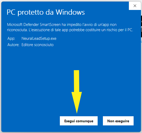
If you see this window, it means that your operating system did not recognize the executable file
In this case just press the underlined More Info
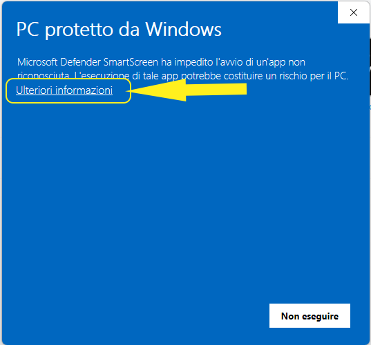
and then Run anyway
Getting Started
NeuralLead Maker is a graphical tool that allows the creation, training and simulation of 3rd generation neural networks (Spike) without using a line of code.
Let's take the first steps within the program to understand the potential
First look
Let's take the first steps within the program to understand the potential
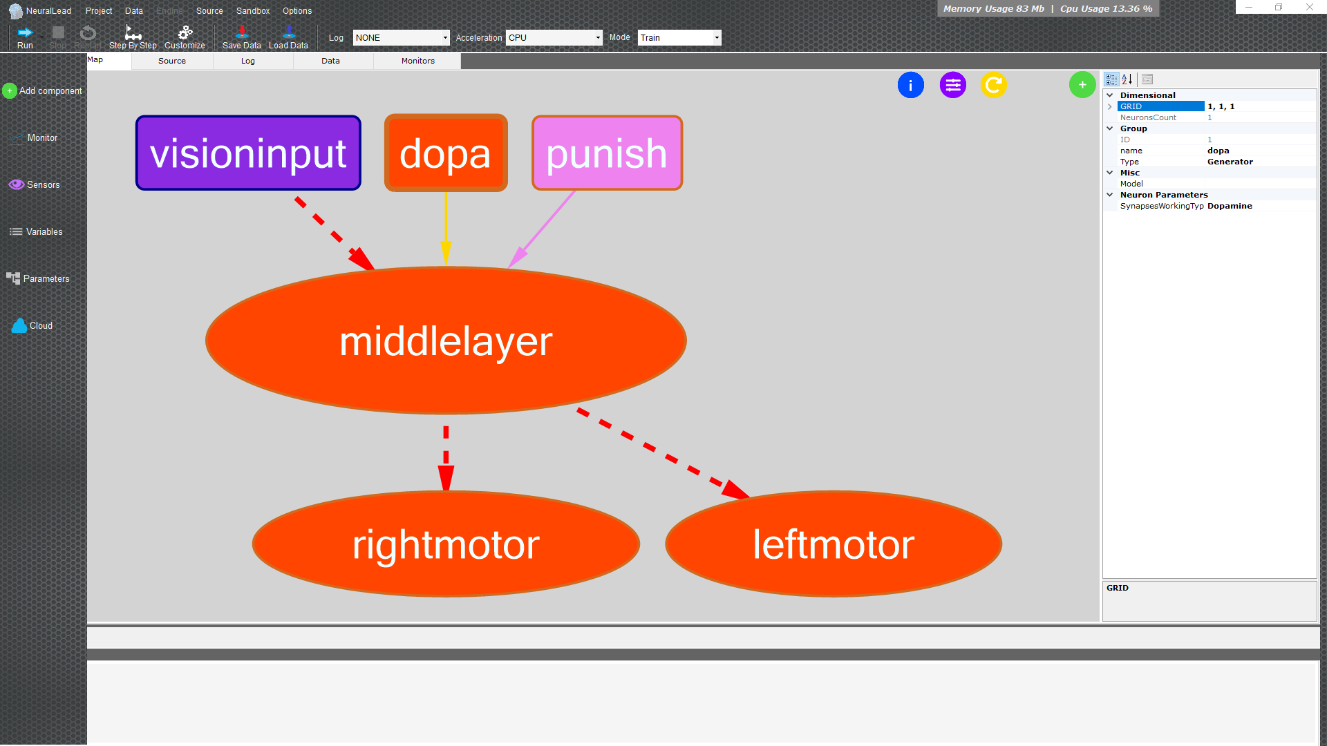
In the left menu we have quick actions to manage the neural network
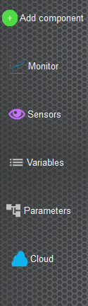
- Add Component that allows you to add parts to the neural network as groups of neural or create a connection between groups of neurons
- Monitors gives the possibility to add elements to record and visualize the information of the neurons or of the connections during the execution of the simulation
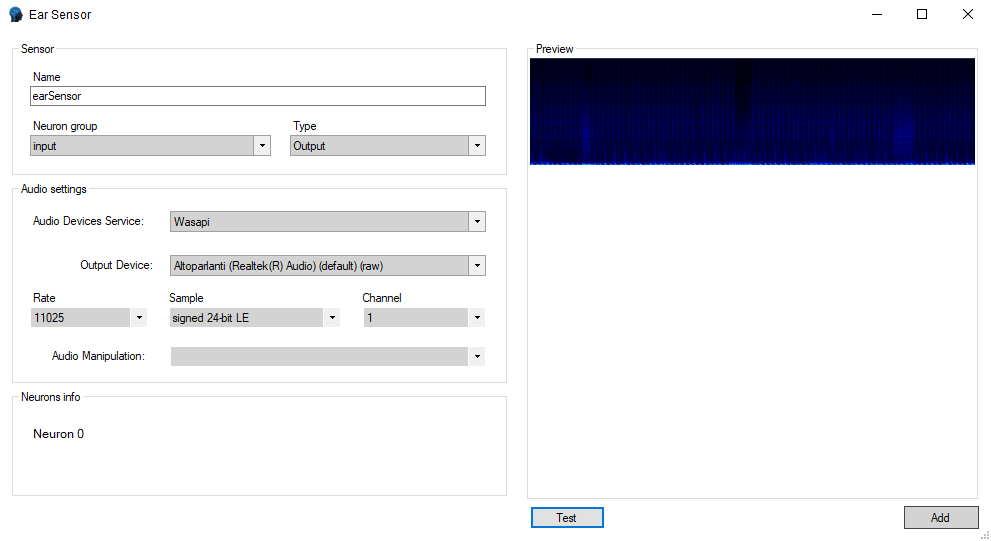
- Sensors is the management of inputs and/or outputs through devices connected to the computer such as webcams, microphones, speakers...
- Variables create, edit, or delete values that are used when creating the neural network
- Parameters quickly visualize all the components of the neural tree network
- Cloud performs actions with the online platform such as synchronizing projects
In the button bar at the top you can control the simulation of the neural network

- Run starts the neural network simulation
- Stop stops the neural network simulation
- Restart stops and restarts the neural network simulation
- Step by Step starts the neural network simulation for one cycle only
- Customize manages generic simulation data, such as the duration of a simulation cycle.
- Save Data saves current neural network data such as neuron voltage values and synaptic weights.
- Load Data loads the previously saved data of the neural network, neurons and synaptic weights.
Be careful not to confuse the save data (SaveData/LoadData), with the project or structure save files.
The project or structure file contains the information to modify the neural network, they are all initial values of neurons, synapses and learning rules, so it is a neural network that needs to be trained.
While the save files contain the information of an already trained neural network, ready for use in your products.
The Pages

- with Brain Map you visualize the components of the neural network (groups of neurons and the connections between them), clicking on the components will show the values in the properties panel
- Source displays the project in XML format
- Log displays the textual output of the running neural network
- Data add, edit, and remove values to assign to neural network inputs and outputs in the form of numeric values
- Monitors allows you to view the enabled monitors such as the graphs of the impulses of the neurons during the execution of the neural network
Brain Map
Click on the blue links to go to advanced information
Group Neurons are the ovals
The background shape of an oval can be
- Viola is a group of Generator neurons that only receives inputs from sensors or other data
- Orange is a group of neurons inside or outside the neural network
Connections are the lines
The shape of the line of a connection between groups of neurons indicates
- The dashed line indicates a plastic connection
- Solid line indicates fixed connection
The colors of the line of a connection between groups of neurons indicates
Yellow dopaminergic connection
By clicking on a group of neurons (colored oval) or on a connection (colored line) it will be possible to see and edit quickly the values that will be shown in the panel on the right
Data
This area allows you to manage the raw input and output data of the neural network.
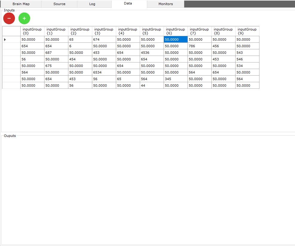
There are 2 types of data:
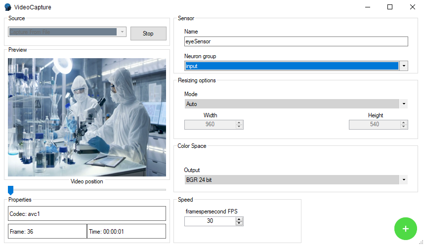
- Sensor data is data from sensors, such as a webcam, a video file, an image dataset, temperature, inputs such as a mouse or keyboard...
- Raw data which is data that is not handled by sensors, it can only be numerical data
Columns like inputGroup {0} or inputGroup {1}... indicate the position of the neuron (0, 1...) within the group of neurons (inputGroup)
Input data rows must be equal to output data rows.
Monitors
View the neural network simulation graphically and quickly
It's not science without a graph
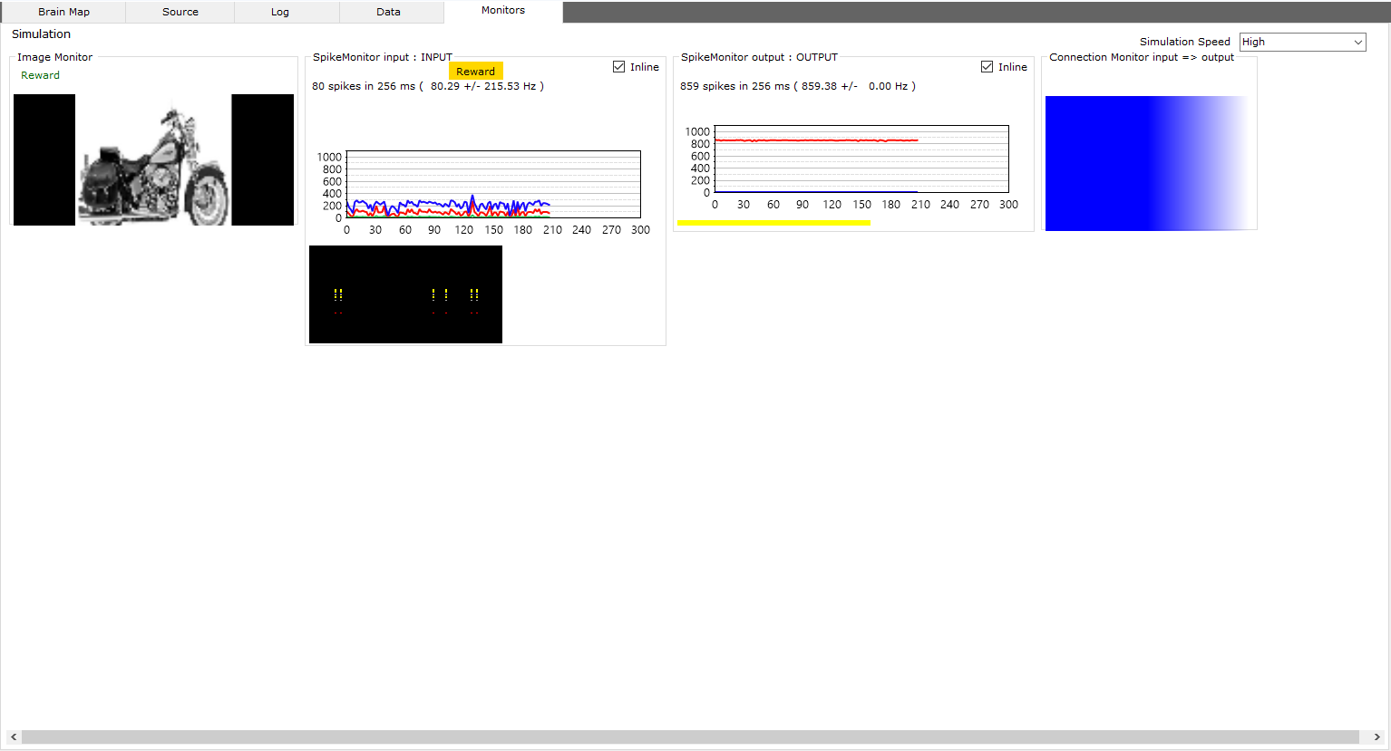
From the monitors and sensors panel in the left menu, activate the monitors and sensors that show the behavior of the neural network during the simulation.
The spike monitor shows the data of the nuron spikes, of the activated group of neurons, occurred within a simulation cycle.
The spikes are shown as a graph or in a plot (colored pixels below the graph)
The chart contains the following colors:
- Red The high frequency (Hz) of the spikes of all neurons within a group
- Blue The low frequency (Hz) of the spikes of all neurons related to the group
- Green The total spike amount for all neurons in a group
The connection monitor shows the data of the synaptic weights of the connections between two groups of neurons
Synaptic weights are shown as a heatmap, cool colors are the weakest synaptic weights compared to warmer colors
All other monitors are related to input / output sensors
Monitors should only be enabled and disabled before or after a simulation, never during a running simulation.
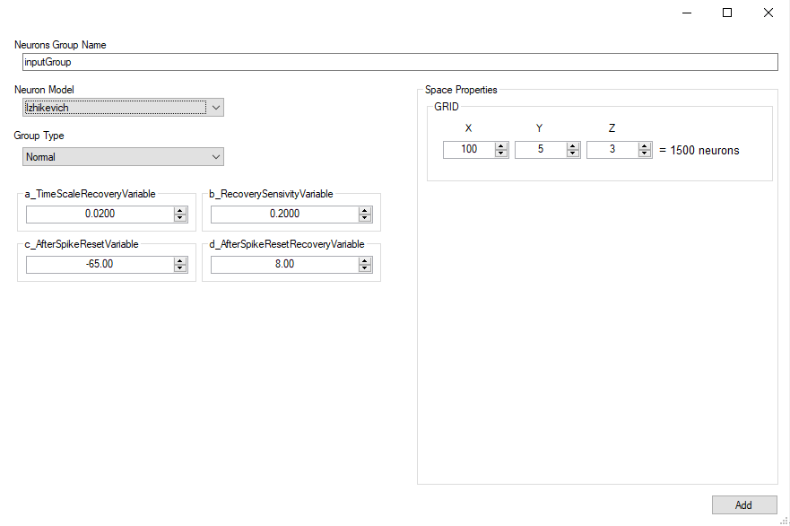
Add Group
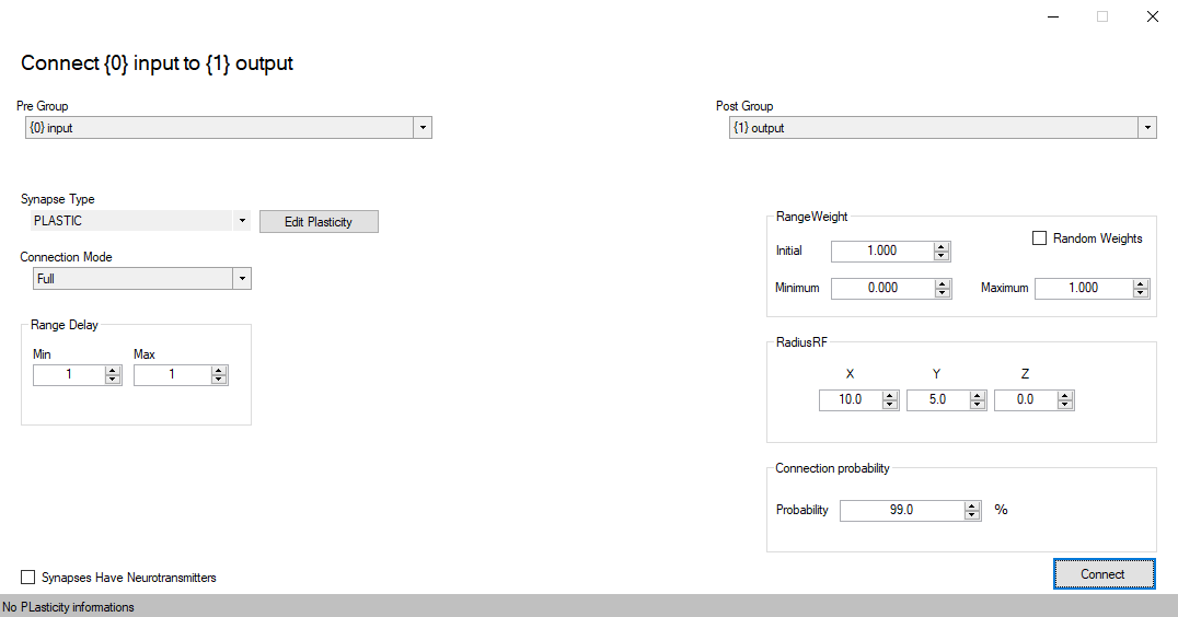
Add Connection
Set plasticity
Classification DataSet
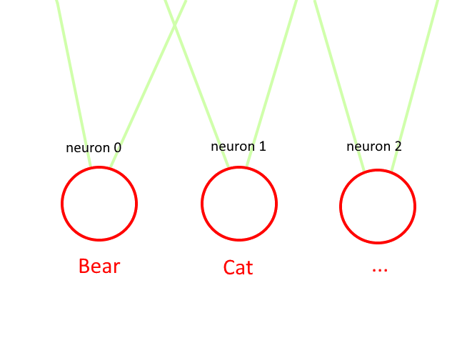
Classification is the process that allows you to globally recognize one image from another,
for example recognizing whether the image looks more like a cat or a bear.
Following the example just mentioned, if there is both a cat and a bear in the image, the neural network returns undefined or inaccurate values.
To work around this inaccuracy you could use an additional cat+bear result as well as just cat and just bear as return values.
It can be deduced that the field of use of the classification method applies to some specific needs, where for example it is necessary to have a generalization of the image.
cat or bear are 2 classes or labels, i.e. the probability that an image belongs to a specific result.
Before proceeding with the creation of the classification DataSet it will be necessary to create a group of input neurons and a group of output neurons and connect them with a plastic connection
Let's proceed by creating our first classification DataSet
- To create the classification datatset (file containing the images linked to the relative classes) it is necessary to open the Data menu of the neurallead application, scroll to local device scroll to images from DataSet... and click on Classification.
- A message will appear asking us if we want to create a new dataset and we will answer Yes.
- At this point it will be necessary to populate our dataset by importing the images of bears and cats by clicking on the first button of the Import toolbar
- Now it is necessary to prepare the dataset with all the possible labels, in our case they are 2 bear and cat, therefore on the right of the window we find an empty list,
above we press the New button and insert the label name
bear. We do the same step for thecat. tag
- As a last step it will be necessary to assign the label (class) to each image, so starting by clicking on the first image that is loaded on the list on the left, once the image is open in the middle of the window, from the toolbar click on Set label to assign the relative class to the loaded image
- Proceed with the last step for all the images found in the image list on the left of the window
Perfect you just created your first classification DataSet with neurallead

Now let's proceed to assign the dataset to a sensor as well as a group of neurons
- Save the DataSet from the toolbar thanks to the Save button and finally close the Classification DataSet window
- The newly created DataSet will automatically be assigned to the training phase, it will be necessary to create a classification dataset also in the testing phase
- Now that we have the dataset for the training phase and one for the testing phase we will need to link the dataset to a Generator group, by selecting from the Input Group listbox
- Finally, we also connect the datasets to a group of output neurons from the Output Group listbox
You have just created a sensor containing training and testing datasets connected to the group of input and output neurons
If during neural network simulation, the first neuron has a higher spike frequency than the other neurons in the output group, then the neural network is saying that the image refers to the first label assigned to the DataSet, if instead the second neuron of the output group a a higher frequency then the neural network is telling you that the image is the second label, and so on...
The connections between the set of assigned inputs and outputs must be plastic, with dopaminergic or non-dopaminergic properties, otherwise there will be no training.
During training all images in the DataSets will be scaled to the amount of neurons in the x and y axis of the neuron group input provided. x = width and y = height of the image
- If you want to process color images, you will need to change the values of
- On the x axis:
x = width * 3andz = 1 - On the z-axis:
x = widthandz = 3 - based on the assignment in the color on neuron axes listbox
The Type of Generator Latency is less energy intensive on hardware resources and usually more effective.
Object Detection DataSet

Camera/Movie and Screen Recorder Sensor
Audio Sensor
Requirements
Your pc should follow these requirements
| Minimum NeuralLead Maker Requirements | |
|---|---|
| Operating System | Windows 8/8.1/10/11
Linux since 2018 Mac OS X 10.14+ |
| CPU | 64 bit 2.2+ GHz with 2 cores |
| GPU | |
| RAM | 4 GB |
| Video Resolution | 1600 x 900 |
| Internet Connection | 100 Mbit/sec |
| NeuralLead Maker recommended requirements | |
|---|---|
| Operating System | Windows 8/8.1/10/11
Linux since 2018 Mac OS X 10.14+ |
| CPU | 64 bit 3.6+ GHz with 8 cores |
| GPU | |
| RAM | 8 GB |
| Video Resolution | 1920 x 1080 |
| Internet Connection | 200 Mbit/sec |
| Minimum NeuralLead Core requirements | |
|---|---|
| Operating System | Windows 8/8.1/10/11
Linux since 2018 Mac OS X 10.14+ Android 5.1+ iOS 11.x+ |
| CPU | 32/64 bit 1 Mhz with 1 core ARM/MIPS/x86/Risc-V |
| GPU | Any or None |
| RAM | 128 MB |
| Video Resolution | Any |
| Internet Connection | Not required |
| Recommended NeuralLead Core requirements | |
|---|---|
| Operating System | Windows 8/8.1/10/11
Linux since 2018 Mac OS X 10.14+ Android 5.1+ iOS 11.x+ |
| CPU | 64 bit 4.2+ GHz with 20 cores |
| GPU | NVidia RTX 3070 |
| RAM | 32 GB |
| Video Resolution | The lowest possible if is on different NeuralLead Maker hardware |
| Internet Connection | 200 Mbit/sec |
How Neural Network Works?
Neurons
The idea is that neurons in the Spiking neural networks is transmit information only when a membrane potential, an intrinsic quality of the neuron related to its membrane electrical charge. Reaches a specific value, called the threshold then do a Spike.
The neuron to reach its threshold follows an algorithm. Each different algorithm creates a different model of neuron.
In the following part there are the different models of neurons and its mathematical formulas
Izhikevich 4 - 2003
The Izhikevich neuron is a dynamical systems model that can be described by a two-dimensional system of ordinary differential equations:

Here, (1) describes the membrane potential v for a given current I, where I is the sum of all synaptic and external currents; that is, I = i_{syn} + I_{ext} (see Synapses). (2) describes a recovery variable u; the parameter a is the rate constant of the recovery variable, and the parameter b describes the sensitivity of the recovery variable to the subthreshold fluctuations of the membrane potential.
All parameters in (1) and (2) are dimensionless; however, the right-hand side of (1) is in a form such that the membrane potential v has mV scale and the time t has ms scale. a, b, c, d are open parameters that have different values for different neuron types.
In contrast to other simple models such as the leaky integrate-and-fire (LIF) neuron, the Izhikevich neuron is able to generate the upstroke of the spike itself.
Thus the voltage reset occurs not at the threshold, but at the peak ( v_{cutoff}=+30 ) of the spike. The action potential downstroke is modeled using an instantaneous reset of the membrane potential whenever v reaches the spike cutoff, plus a stepping of the recovery variable:

The inclusion of u in the model allows for the simulation of typical spike patterns observed in biological neurons.
The four parameters a, b, c, d can be set to simulate different types of neurons.
For example, regular spiking (RS) neurons (class 1 excitable) have a=0.02, b=0.2, c=-65, d=8.
Fast spiking (FS) neurons (class 2 excitable) have a=0.1, b=0.2, c=-65, d=2).
For more information on different neuron types, see Izhikevich (2003, 2004).
Izhikevich 9 - 2007
The 9-parameter izhikevich neuron model is equivalent to the 4-parameter one. Larger number of parameters is used for convenience in describing various neuron types.

Here, (5) describes the membrane potential v for a given current I, where I is the sum of all synaptic and external currents; that is, I = i_{syn} + I_{ext} (see Synapses).
The parameter k is a rate constant of the membrane potential, and can be found using the rheobase and the input resistance of a neuron. The parameter vr is the resting membrane potential. The parameter vt is the instantaneous threshold potential. The parameter C is the membrane capacitance.

Here, (15) describes a recovery variable u;
The parameter a is the rate constant of the recovery variable. The parameter b describes the sensitivity of the recovery variable to the subthreshold fluctuations of the membrane potential. The parameter vr is the resting membrane potential.
All parameters in (5) and (6) are dimensionless; however, the right-hand side of (5) is in a form such that the membrane potential v has mV scale and the time t has ms scale. is voltage, u is the recovery variable, I is the input current, and C, k, vr, vt, a, b, vpeak, c, d are open parameters that have different values for different neuron types.
In contrast to other simple models such as the leaky integrate-and-fire (LIF) neuron, the Izhikevich neuron is able to generate the upstroke of the spike itself. Thus the voltage reset occurs not at the threshold, but at the peak ( v_{cutoff}=+vpeak ) of the spike. The action potential downstroke is modeled using an instantaneous reset of the membrane potential whenever v reaches the spike cutoff, plus a stepping of the recovery variable:

Regular spiking (RS) neurons (class 1 excitable) have C=100, k=0.7, vr=-60, vt=-40, a=0.03, b=-2.0, vpeak=35, c=-50, d=100.
Fast spiking (FS) neurons (class 2 excitable) have C=20, k=1, vr=-55, vt=-40, a=0.15, b=8, vpeak=25, c=-55, d=200).
For more information on different neuron types, see Izhikevich (2003, 2004). For more information about 9-parameter model see Izhikevich (2007).
LIF - Leaky Integrate and Fire
Leaky integrate and fire (LIF) model represents neuron as a parallel combination of a “leaky” resistor (conductance, g L ) and a capacitor (C) as shown in Fig. 2(a). A current source I(t) is used as synaptic current input to charge up the capacitor to produce a potential V(t).
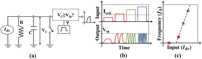
(a) LIF neuron circuit model, (b) For input (Idc < Icrit), V(t) never exceeds Vth- hence neuron never spikes. However, for Idc ≥ Icrit, neuron will fire when V(t) ≥ Vth and immediately reset i.e. V(t) = EL, (c) With higher input (e.g. Idc ≥ Icrit), firing rate or the frequency increases like a biological neuron while for low input (Idc < Icrit), frequency is zero. The output frequency (fo) vs. input is the signature neuronal function to be mimicked artificially.
When potential exceeds threshold (V(t) ≥ V th ), the capacitor discharges to a resting potential E L using the voltage-controlled switch, like a biological neuron. Each time LIF neuron voltage exceeds threshold, a separate driver circuit (say, D3) issues a spike as mentioned in the last section. Thus, LIF model is governed by the following differential equation:
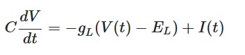
At low input current (I(t)), V(t) never exceeds threshold V th - which produces no spikes (i.e. t i → ∞). For example, if a dc input (i.e. I(t) = I dc ) does not exceed a critical current (I crit = g L (V th − E L )), V(t) will always be less than V th (i.e. V(t) < V th ), by simple steady state analysis of Eqn. 1. When I(t) is high (e.g. I dc > I crit ), the charge up time to V th reduces (Fig. 2b). This essentially increases the output frequency (f o ) with increase in input I dc (Fig. 2c).
Huxley Hodgkin
It is a set of nonlinear differential equations that approximates the electrical characteristics of excitable cells such as neurons and cardiac myocytes. It is a continuous-time dynamical system.
Alan Hodgkin and Andrew Huxley described the model in 1952 to explain the ionic mechanisms underlying the initiation and propagation of action potentials in the squid giant axon. They received the 1963 Nobel Prize in Physiology or Medicine for this work.
Comparisons
| Neuron Model | Biological Plausibility | Performances CPU/GPU |
| Huxley Hodgkin | Very High | Low |
| Izhikevich 4 - 2003 | Low | High |
| Izhikevich 9 - 2007 | High | Low |
| Leaky Integrate and Fire | Very Low | Very High |
Synapses
Spiking neural networks deliver information beetwen neurons using spikes via structures called synapses.
In biology, synapses pass information from one neuron to another via a chemical signal (electrical synapses also exist).
Communication between synapses is, in general, unidirectional.
Synapses are broken into two components: one component located on the neuron sending the information (the presynaptic neuron) and one component located on the neuron receiving the information (the postsynaptic neuron).
The two synapse components are separated by a physical gap between the pre and postsynaptic neurons called the synaptic cleft. Information is passed from the presynaptic neuron to the postsynaptic neuron when the presynaptic component of the synapse releases neurotransmitters that cross the synaptic cleft and bind to postsynaptic receptors that result in a current influx into the postsynaptic neuron.
The sum of many synaptic current contributions change the postsynaptic neuron voltage, causing it to spike if the voltage threshold is crossed.
NeuralLead supports two synapse model descriptions. The current-based description uses a single synaptic current term while the conductance-based description calculates the synaptic current using more complex conductance equations for each synaptic receptor-type. Conductance/current mode contributions are influenced by the synaptic weight of the synapse.
Current transmission
When current based (CUBA) mode is used, no conductances are present. The strength of the resulting current is directly proportional to the synaptic weight. Additionally, the total synaptic current at postsynaptic neuron j, I_{j}^{syn} , due to a spike from presynaptic neuron i is given at any point in time by (5):

where s_{ij} is 1 if the neuron is spiking and 0 otherwise, w_{ij} is the strength of the synaptic weight between postsynaptic neuron j and presynaptic neuron i, and N is the total amount of presynaptic connections onto postsynaptic neuron j.
Current mode is the default behavior of all neurons. NeuralLead full support mixed modes consisting of some neurons with conductances and others without conductances in the same simulation.
Because Current mode has synaptic currents that last for a single time step, and Conductances mode has synaptic currents that decay over time, switching from Current mode to Conductance mode usually requires the user to reduce the synaptic weights as the resulting currents will be much larger in Conductance mode.
Conductance (Neurotransmitters) transmission
When conductance-based mode is used, there are conductances with exponential decays present. If the synaptic connection is excitatory then AMPA and NMDA decay values are used.
If the synaptic connection is inhibitory then GABA A and GABA B decay values are used. Equation (6) shows the corresponding current, I_{ij} in postsynaptic neuron j, due to inputs from N presynaptic neurons (denoted by i).

Here we drop the i,j notation and assume the g values pertain to a specific synapse ( i,j ) and the v values pertain to a specific postsynaptic neuron, j. The total current from a particular synapse can either be excitatory ( i_{e} ) or inhibitory ( i_{i} ). They are described in equations (7) and (8), below:

The excitatory current is comprised of an AMPA current ( i_{AMPA} ) and a voltage dependent NMDA current ( i_{NMDA} ). They are described in equations (9) and (10).
Here, g is the conductance, v is the postsynaptic voltage, and v^{rev} is the reversal potential. Both g and v^{rev} are specific to a particular ion channel/receptor. The inhibitory current is comprised of a GABA A current ( i_{GABA_A} ) and a GABA B current ( i_{GABA_B} ) shown in equations (11) and (12).

The conductance, g, for each ion channel/receptor, k is given in the general form equation (13).

Where f indicates a particular spike event, t_f represents the time of this spike event, and \Theta is the Heaviside function.
Default values can be decay_AMPA=5ms, decay_NMDA=150ms, decay_GABAa=6ms, decay_GABAb=150ms
Neurons Group
A group contains neurons distributed in a space in 1, 2 or 3 dimensions.
Space
Neurons in a group can be arranged into a (up to) three-dimensional (primitive cubic) grid using the Grid struct, and connections can be specified depending on the relative placement of neurons. This allows for the creation of networks with complex spatial structure.
Each neuron in the group gets assigned a (x,y,z) location on a 3D grid centered around the origin, so that calling Grid(Nx,Ny,Nz) creates coordinates that fall in the range [-(Nx-1)/2, (Nx-1)/2], [-(Ny-1)/2, (Ny-1)/2], and [-(Nz-1)/2, (Nz-1)/2].
The resulting grid is a primitive cubic Bravais lattice with cubic side length 1 (arbitrary units). The primitive (or simple) cubic crystal system consists of one lattice point (neuron) on each corner of the cube. Each neuron at a lattice point is then shared equally between eight adjacent cubes.
An example is shown in the figure below.
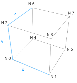
The 3D grid generated by Grid(2,2,2). Black circles indicate the 3D coordinates of all the neurons (with corresponding neuron positions) in the group.
Examples
Grid(1,1,1)will create a single neuron with location (0,0,0).Grid(2,1,1)will create two neurons, where the first neuron (N 0) has location (-0.5,0,0), and the second neuron (N 1) has location (0.5,0,0).Grid(1,1,2)will create two neurons, where the first neuron (N 0) has location (0,0,-0.5), and the second neuron (N 1) has location (0,0,0.5).Grid(2,2,2)will create eight neurons, where the first neuron (N 0) has location (-0.5,-0.5,-0.5), the second neuron has location (0.5,-0.5,-0.5), the third has (-0.5,0.5,-0.5), and so forth (see figure below).Grid(3,3,3)will create 3x3x3=27 neurons, where the first neuron (N 0) has location (-1,-1,-1), the second neuron has location (0,-1,-1), the third has (1,-1,-1), the fourth has (-1,0,-1), ..., and the last one has (1,1,1).
Connections
Connections connect groups of neurons with synapses, allowing the passage of information.
A connection can selectively connect neurons between groups, forcing impulses of a neuron to take a path between synapses.
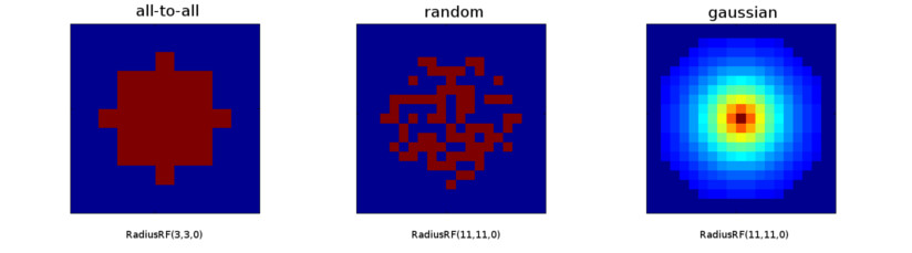
There are a number of pre-defined connection types, as All-to-all, random, one-to-one, and Gaussian connectivity.
All-to-all (also known as "full") connectivity connects all neurons in the pre-synaptic group to all neurons in the post-synaptic group (with or without self-connections).
One-to-one connectivity connects neuron i in the pre-synaptic group to neuron i in the post-synaptic group (both groups should have the same number of neurons).
Random connectivity connects a group of pre-synaptic neurons randomly to a group of post-synaptic neurons with a user-specified probability p.
Gaussian connectivity uses topographic information from the Grid struct to connects neurons based on their relative distance in 3D space.
The RangeWeight Struct
RangeWeight is a struct that simplifies the specification of the lower bound Minimum and upper bound Maximum of the weights as well as an initial weight value Initial. For fixed synapses (no plasticity) these three values are all the same. This will set all fields of the struct to value wt.
On the other hand, plastic synapses are initialized to Initial, and can range during smulation between Minimum and Maximum
In plastic synapses, if the Randomize property is enabled, the synapses will have a random initial value between the Initial and Maximum values. If the Randomize property is disabled the initial synaptic connection will be equal to Initial for all synapses in the connection
Note that all specified weights are considered weight magnitudes and should thus be non-negative, even for inhibitory connections.
The RangeDelay Struct
Similar to RangeWeight, RangeDelay is a struct to specify the lower bound Minimum and upper bound Maximum of a synaptic delay range.
Synaptic delays are measured in milliseconds, and can only take integer values.
Example RangeDelay.Minimum = 1 and RangeDelay.Maximum = 20, means synaptic delays that are uniformly distributed between 1ms and 20ms
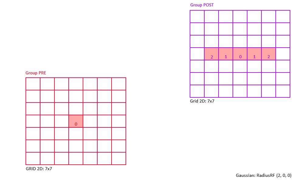
Radius Receptive Field (RadiusRF) Struct
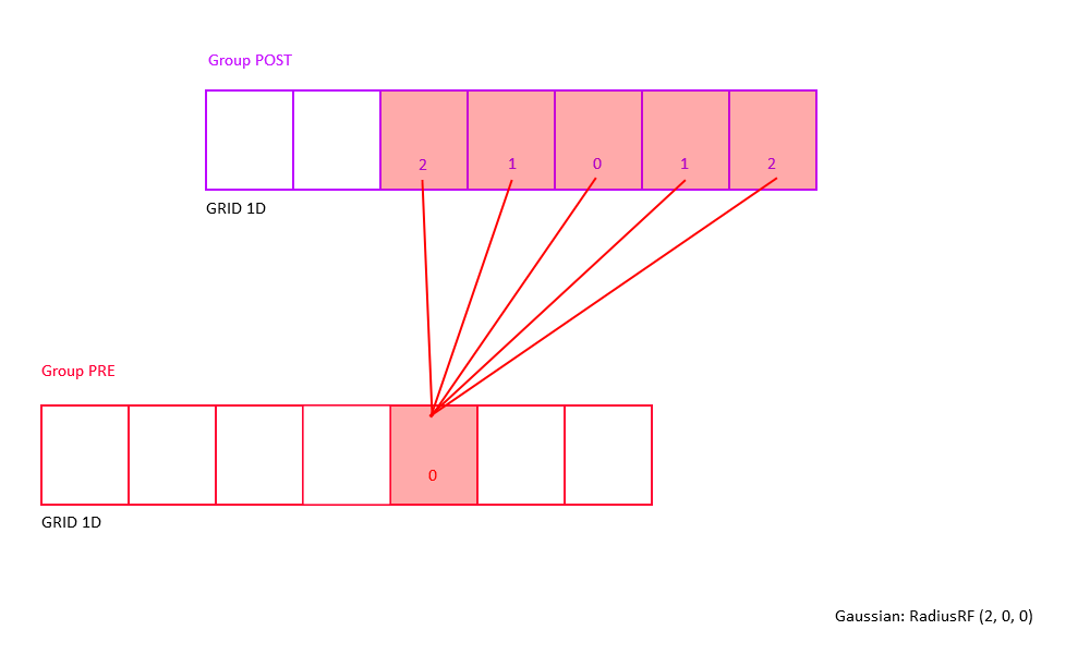
Each connection type can make use of an optional RadiusRF struct to specify circular receptive fields (RFs) in 1D, 2D, or 3D, following the topographic organization of the Grid struct (see Topography. This allows for the creation of networks with complex spatial structure.
Spatial RFs are always specified from the point of view of a post-synaptic neuron at location (post.x, post.y, post.z), looking back on all the pre-synaptic neurons at location (pre.x, pre.y, pre.z) it is connected to.
Using the Grid struct, neurons in a group can be arranged into a (up to) three-dimensional (primitive cubic) grid with side length 1 (arbitrary units). Each neuron in the group gets assigned a (x,y,z) location on a 3D grid centered around the origin, so that calling Grid(Nx,Ny,Nz) creates coordinates that fall in the range [-(Nx-1)/2, (Nx-1)/2], [-(Ny-1)/2, (Ny-1)/2], and [-(Nz-1)/2, (Nz-1)/2]. For more information on the Grid struct, please refer to Topography.
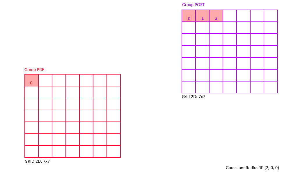
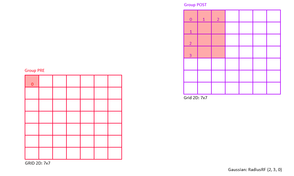
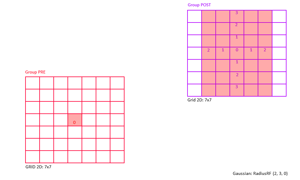
The RadiusRF struct follows the spatial arrangement (and arbitrary units) established by Grid. The struct takes up to three values, which specify the radius of a circular receptive field in x, y, and z. If the radius in one dimension is 0, say RadiusRF.radX==0, then pre.x must be equal to post.x in order to be connected. If the radius in one dimension is -1, say RadiusRF.radX==-1, then pre and post will be connected no matter their specific pre.x and post.x Otherwise, if the radius in one dimension is a positive real number, the RF radius will be exactly that number.
Examples
- Create a 2D Gaussian RF of radius 10 in z-plane:
RadiusRF(10, 10, 0)Neuron pre will be connected to neuron post iff(pre.x-post.x)^2 + (pre.y-post.y)^2 <= 100andpre.z==post.z. - Create a 2D heterogeneous Gaussian RF (an ellipse) with semi-axes 10 and 5:
RadiusRF(10, 5, 0)Neuron pre will be connected to neuron post iff(pre.x-post.x)/100 + (pre.y-post.y)^2/25 <= 1andpre.z==post.z. - Connect all to all, no matter the RF (default):
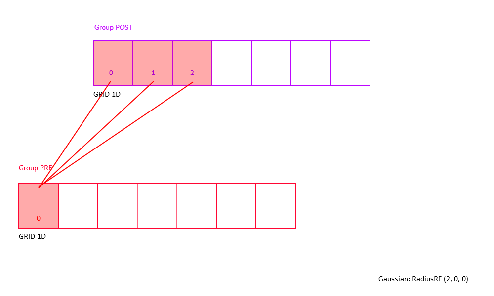
RadiusRF(-1, -1, -1) - Connect one-to-one:
RadiusRF(0, 0, 0)Neuron pre will be connected to neuron post iffpre.x==post.x, pre.y==post.y, pre.z==post.z. Note: Use connection type "one-to-one" instead.
Synaptic Gain Factors
In conductance mode synaptic receptor-specific gain factors can be specified to vary the neurotransmitters.
Indicate a multiplicative gain factor for fast and slow synaptic channels.
| Fast Channel | Slow Channel | |
|---|---|---|
| Excitatory | AMPA | NMDA |
| Inhibitory | GABA a | GABA b |
Full Connectivity
All-to-all (also known as "full") connectivity connects all neurons in the pre-synaptic group to all neurons in the post-synaptic group (with or without self-connections).
Full-No-Direct Connettivity
Alternatively, one can use the "full-no-direct" keyword to indicate that no self-connections shall be made:
Connect pre neuron to all post neurons and will prevent neuron in the pre-synaptic group to be connected to neuron in the same x,y, and z 3D post-synaptic group position.
Random Connectivity
Random connectivity connects a group of pre-synaptic neurons randomly to a group of post-synaptic neurons with a user-specified probability from 0 to 100%.
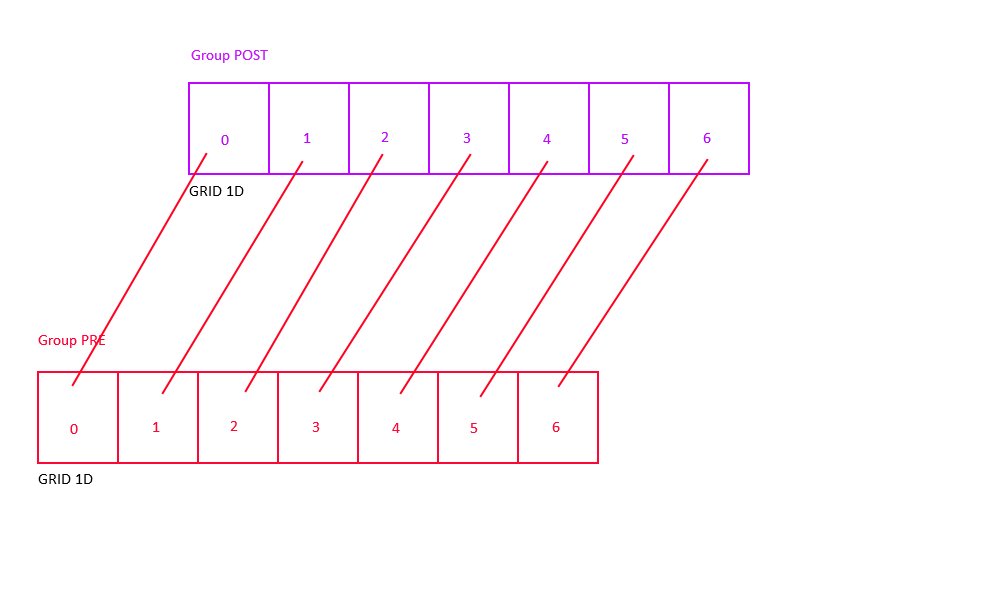
One-to-One Connectivity
One-to-one connectivity connects neuron i in the pre-synaptic group to neuron i in the post-synaptic group (both groups should have the same number of neurons).
In order to achieve topographic one-to-one connectivity (i.e., connect two neurons only if they code for the same spatial location), use Gaussian connectivity with RadiusRF(0,0,0).
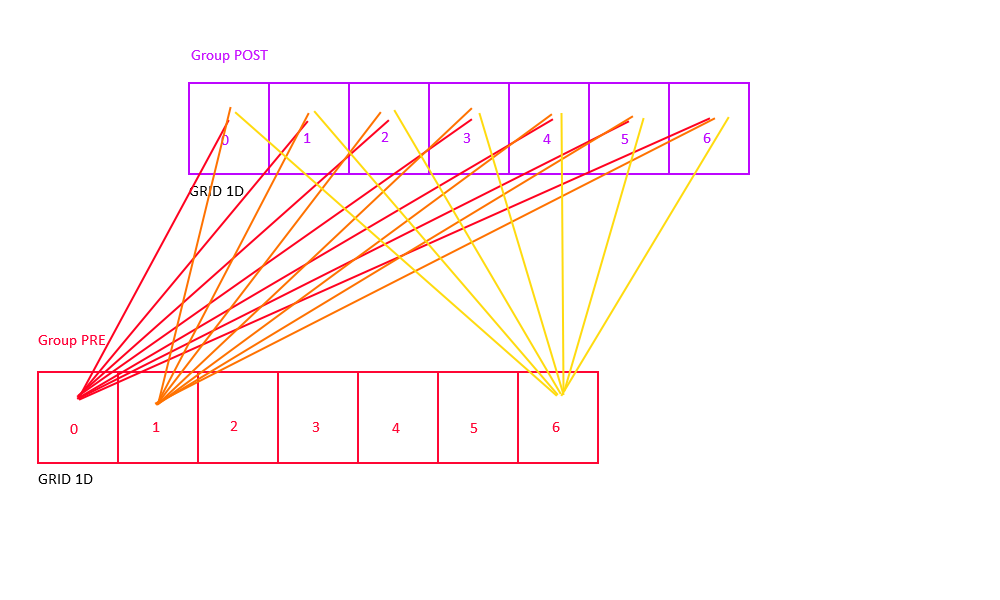
Gaussian Connectivity
Gaussian connectivity uses topographic information from the Grid struct to connect neurons based on their relative distance in 3D space. The extent of the Gaussian neighborhood is specified via the RadiusRF struct, which accepts three parameters to specify a receptive field radius in dimensions x, y, and z. This makes it possible to create 1D, 2D, or 3D circular receptive fields.
RangeWeight(0.25f), Probability(100%), RangeDelay(1), RadiusRF(10,10,0), FIXED SYNAPSE
RangeWeight is a struct that simplifies the specification of minimum, initial, and maximum weight values; and in this case it specifies the maximum weight value, which is achieved when both pre-synaptic and post-synaptic neuron code for the same spatial location. The next parameter, 1.0f, sets the connection probability to 100%. RadiusRF(10,10,0) specifies that a 2D receptive fields in x and y shall be created with radius 10 (see example below). Setting radius in z to 0 forces neurons to have the exact same z-coordinate in order to be connected.
A few things should be noted about the implementation. Usually, one specifies the Gaussian width or standard deviation of the normal distribution (i.e., the parameter sigma). Here, in order to standardize across connection types, the Gaussian width is instead inferred from the RadiusRF structs, such that neurons at the very border of the receptive field are connected with a weight that is 10% of the maximum specified weight. Within the receptive field weights drop with distance squared, as is the case with a regular normal distribution. Note that units for distance are arbitrary, in that they are not tied to any physical unit of space. Instead, units are tied to the Grid struct, which places consecutive neurons 1 arbitrary unit apart.
Example: Consider a 2D receptive field RadiusRF(a,b,0).
Here, two neurons "pre" and "post", coding for spatial locations (pre.x, pre.y, pre.z) and (post.x, post.y, post.z),
will be connected (pre.x-post.x)^2/a^2 + (pre.y-post.y)/b^2 <= 1 (which is the ellipse inequality) and pre.z==post.z.
The weight will be maximal (i.e., RangeWeight.Maximum) if "pre" and "post" code for the same (x,y) location.
Within the receptive field, the weights drop with distance squared, so that neurons for which (pre.x-post.x)^2/a^2 + (pre.y-post.y)/b^2 == 1 (exactly equal to 1) are connected with 0.1*RangeWeight.Maximum.
Outside the receptive field, weights are zero.
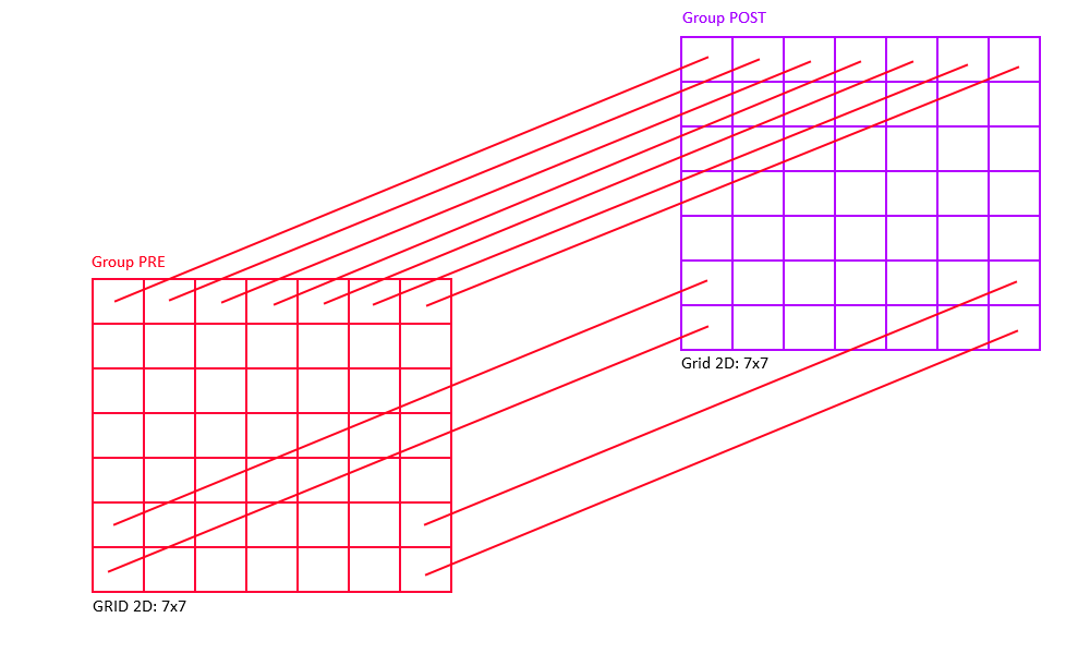
Another case to consider is where the presynaptic and postsynaptic group have different Grid structs (or consist of different numbers of neurons).
In order to cover the full space that these groups cover, the coordinate of the presynaptic group will be scaled to the dimensions of the postsynaptic group: pre.x = pre.x / gridPre.x * gridPost.x, pre.y = pre.y / gridPre.y * gridPost.y, and pre.z = pre.z / gridPre.z * gridPost.z.
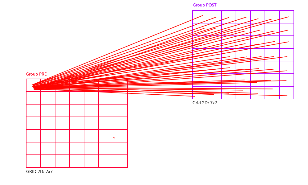
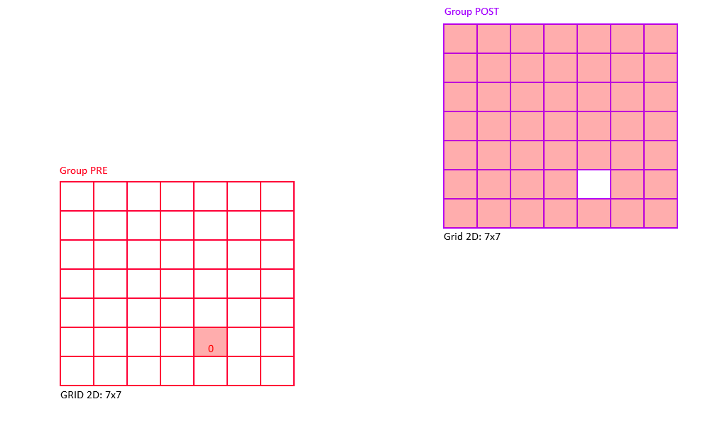
Examples of 2D Gaussian receptive fields (topographic heatmap of weight strengths).
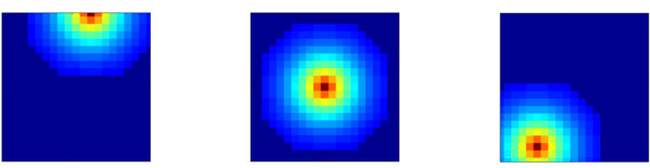
The following figures shows some of examples of a 2D Gaussian receptive field created with RadiusRF(9,9,0).
Each panel shows the receptive field of a particular post-synaptic neuron (coding for different spatial locations) looking back at its pre-synaptic connections.
By making use of the flexibility that is provided by the RadiusRF struct, it is possible to create any 1D, 2D, or 3D Gaussian receptive field.
A few examples that are easy to visualize are shown in the figure below.
The first panel is essentially a one-to-one connection by using RadiusRF(0,0,0).
But, assume you would want to connect neurons only if their (x,y) location is the same, but did not care about their z-coordinates.
This could simply be achieved by using RadiusRF(0,0,-1).
Similary, it is possible to permute the x, y, and z dimensions in the logic.
You could connect neurons according to distance in y, only if their z-coordinate was the same, no matter the x-coordinate: RadiusRF(-1,y,0).
Or, you could connect neurons in a 3D ellipsoid: RadiusRF(a,b,c).
RadiusRF and Grid use the same but arbitrary units, where neurons are placed on a (primitive cubic) grid with cubic side length 1, so that consecutive neurons on the grid are placed 1 arbitrary unit apart.
Any 1D, 2D, or 3D Gaussian receptive field is possible. However, visualization is currently limited to 2D planes.
Since the Gaussian width is inferred from receptive field dimensions, using "gaussian" connectivity in combination with RadiusRF(-1,-1,-1) is not allowed.
Pool Connettivity
Topographically the same of gaussian, but the Z of RadiusRF is ever 0. Connection weight not follow a radius, but initial min and maximum parameters.
Convolutional Connettivity
Topographically the same of gaussian, but the Z of RadiusRF is ever -1, then the connection is repeated in 2D for each z-axis of the post group. Connection weight not follow a radius, but all connection in the same z has the same initial connection weight value.
Reverse Connettivity
For each connection shown above, there is a chance to reverse the connections between the pre synaptic group and the post synaptic group.
For example with full connectivity inversion, the first neuron of the pre group will be connected to the last neuron of the post group.
The same also applies to the type of connectivity Random, Gaussian, One-to-One or Pool, ie the first of the pre to the last of the post, the second neuron of the pre to the second of the post and so on.
Synaptic Plasticity
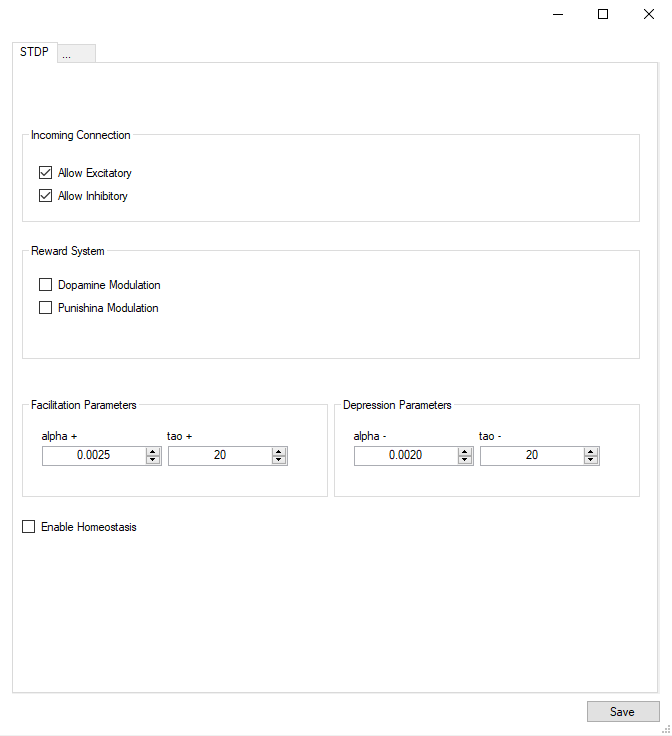
Spike-Timing Dependent Plasticity (STDP)
A popular spike-based learning phenomenon called spike-timing dependent plasticity (STDP). STDP is an important form of Hebbian learning where the precise timing of the pre and postsynaptic spike times influence synaptic weight changes. STDP is important because it operates on correlations between spikes and suggests a potential causal (or anti-causal) relationship between pre and postsynaptic spikes (Sjöström and Gerstner, 2010).
The prototypical form of STDP acts as follows: spike-timings where the presynaptic spike arrival precedes postsynaptic spikes by a few milliseconds results in an increase in the synaptic weight, also referred to as long-term potentiation (LTP). Spike-timings where the presynaptic spike arrival follows postsynaptic spikes by a few milliseconds result in a decrease in the synaptic weight. (Bi and Poo, 1998). STDP of this type was observed at glutamatergic (excitatory) synapses.
Phenomenological Model of STDP
Fig. 2 shows a variety of 'STDP Curves' possible using NeuralLead. In each sub-figure, the horizontal axis represents the time difference between the time of the presynaptic spike arrival and the time of the postsynaptic arrival or Delta t = t_{post} - t_{pre}. Therefore, Delta t's to the left of the vertical axis are Delta t < 0 (pre-after-post) while Delta t's to the right of the vertical axis are Delta t>0 (pre-before-post). The vertical axis represents the weight change of the synaptic weight magnitude Delta \vert w \vert at that synapse.
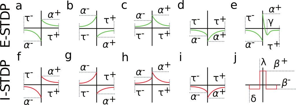
Fig. 2. Examples of possible STDP curves possible in NeuralLead. Green curves can be applied to glutamatergic synapses, whereas red curves can be applied to GABAergic (inhibitory) synapses.STDP (2(a)-2(d)) and (2(f)-2(i)). are referred to as STDP type ExpCurve as they consist of two decaying exponentials. 2(e) is referred to as STDP type PulseCurve 2(j).
If Delta t > 0, then Delta w = A_{+} \exp(-\Delta t/\tau_{+}) else if Delta t <= 0, then Delta w = A_{-} \exp(-\Delta t/\tau_{-}).
the A_{+} and A_{-} parameters appropriately as these parameters are allowed to take both positive and negative values. Users also select the tau_{+} and tau_{-} exponential decay parameters.
The change in weights is calculate with the following equation:

where w_{i,j} is the weight from presynaptic neuron i, to postsynaptic neuron j, delta is a bias with a default value of 0, and beta is the learning rate with a default value of 1. Additionally, \mbox{pre-before-post}_{i,j} is the pre-before-post weight change contribution and \mbox{pre-after-post}_{i,j} is the pre-after-post weight change contribution.
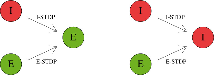
STDP type by both STDP weight change curve (as shown in Fig. 2) and by type of synaptic connection (e.g. excitatory or inhibitory). As mentioned in previous chapters, excitatory synapses bring the postsynaptic neuron closer to its firing threshold while inhibitory synapses bring the postsynaptic neuron away from its firing threshold. The combination of STDP weight change curve and synapse type have functional implications for the neural circuit being constructed. E-STDP is defined as STDP on a connection where the presynaptic neuron groups are excitatory in nature. This is true for E to E and E to I connections. I-STDP is defined as STDP on a connection where the presynaptic neuron groups are inhibitory in nature. Fig. 3 shows illustrates how E-STDP and I-STDP are defined.
You cannot apply any learning rules with connections of type Fixed. Use plastic connections instead.
Excitatory STDP (Exc-STDP) and Inhibitory STDP (Inh-STDP)
The possible types of E-STDP curves are shown in the top row of Fig. 2. The presynaptic group determines the identity of the STDP type (E-STDP or I-STDP). Currently NeuralLead supports one set of unique STDP parameters for per STDP type. Therefore, in Fig. 3, the I to E and E to E plastic connections to the exctiatory neuron on the left could have completely different STDP curves (shown in Fig. 2). However, if a third connection were added, like another E to E connection, then STDP parameter values for that E to E connection must be identical to that of the other E to E connection.
Dopamine-Modulated STDP
Dopamine-modulated STDP implementation allows users to easily implement reinforcement learning applications. Dopamine acts as a training signal in the sense that STDP only takes place in the presence of elevated dopamine concentrations. Below is a code snippet that implements dopamine-modulated STDP.
Homeostasis
Disabling Plasticity in Testing Phase
NeuralLead provides a method to temporarily disable all synaptic weight updates, which may be helpful in a testing phase that is trying to evaluate some previously trained network.
Microglia Cell
A very important part of learning that is overlooked in other neural network simulators are Gliar cells.
A very important part of learning that is overlooked in other neural network simulators are Gliar cells.
Gliar cells allow for very dynamic training, pruning dead neurons and synapses, and gliar cells are also capable of creating new synapses.
The creation of new synapses is very important because it allows you to change the structure of the brain and improve its training.
The activation of the glial cells can be activated or deactivated for the whole neural network, furthermore if activated it is necessary to establish a value in milliseconds which indicates how often the microglia cells prune the dead cells (neurons and synapses).
If a neuron no longer has presynaptic connections it is considered unusable because it can no longer receive any type of input signal, therefore it is considered dead and the glia cells can remove the dead neurons because they are useless. Also consider that new presynaptic connections can be made to dead neurons and then they can come back to life.
With neurallead you can set the values of gliary cells to act on:
- Synapse Elimination On/Off
- Delete Neurons On/Off
- How many steps or cycles glial cells activate to clean
Inputs
A Generator allows you to set values to neurons in groups assigned as input.
Since for neural networks Spikes can only have digital values 0 or 1, to integrate higher values it is necessary to distribute the 1s and 0s over time.
There are several ways or classes to associate inputs over time, let's look at the classes that NeuralLead integrates.
Rate Class
The rate class defines to distribute a value in a given time, creating oscillations in the time period with moments of rest if the input at that moment is 0.
For example, if the input value is equal to 10 and a simulation cycle is equal to 50 milliseconds. 10 pulses of 5 ms duration will be sent for each pulse with 5 ms rest which will be equally distributed every 50 milliseconds.
For the more experienced, the duty cycle is fixed at 50%.
In this example it will not be possible to assign an input Rate greater than 50, because the duration of the cycle is 50 milliseconds, therefore to assign a higher Rate it will be necessary to increase the duration by one cycle.
Latency Class
The Latency class instead is able to assign an input value that refers to the beginning of the activation of the neuron at the established millisecond within the cycle up to the end of the current cycle.
Example: If the input for neuron 1 is equal to 50 and the duration of a cycle is 150 milliseconds, the input will behave with an initial silence (zero neuron spike) of 50 milliseconds and from the 50th millisecond the neuron will continue to spike until the end of the 150 millisecond.
NeuralLead Virtual Shared Host
Download
Follow these instructions to download NeuralLead Maker
- To install NeuralLead VSH you need to log in (or register) on the cloud portal at www.cloud.neurallead.com
- In the left menu select NeuralLead > Rent My Machine
- Press Calculate your earning executable file
- If your earning is positive, a green button will be shown to download the program. Press it.
- Click on your operating system logo
- A modal will open with the libraries to install.
- Restart the operating system
- Start SJR.NeuralLead.VirtualSharedHost.exe or in linux open terminal and type cd /home/$USER/VSH && mono SJR.NeuralLead.VirtualSharedHost.exe
- The first time you open VSH, accept or decline the licenses and enter your NeuralLead.com cloud credentials
- If everything went well, you will see the message Machine Started!
Please note that from Rent My Machine cloud web page, you can check the status of your machines at any time.